Tensor products of vector spaces, part 1

A little while back on this blog, we defined the free k-vector space over a type b:

newtype Vect k b = V [(b,k)] deriving (Eq,Ord)
Elements of Vect k b are k-linear combinations of elements of b.

Whenever we have a mathematical structure like this, we want to know about building blocks and new-from-old constructions.

We already looked at one new-from-old construction: given free k-vector spaces A = Vect k a and B = Vect k b, we can construct their direct sum A⊕B = Vect k (Either a b).

We saw that the direct sum is both the product and the coproduct in the category of free vector spaces - which means that it is the object which satisfies the universal properties implied by the following two diagrams:

So we have injections i1, i2 : Vect k a, Vect k b -> Vect k (Either a b), to put elements of A and B into the direct sum A⊕B, and projections p1, p2 : Vect k (Either a b) -> Vect k a, Vect k b to take them back out again.


However, there is another obvious new-from-old construction: Vect k (a,b). What does this represent?

In order to answer that question, we need to look at bilinear functions. The basic idea of a bilinear function is that it is a function of two arguments, which is linear in each argument. So we might start by looking at functions f :: Vect k a -> Vect k b -> Vect k t.

However, functions of two arguments don't really sit very well in category theory, where arrows are meant to have a single source. (We can handle functions of two arguments in multicategories, but I don't want to go there just yet.) In order to stay within category theory, we need to combine the two arguments into a single argument, using the direct sum construction. So instead of looking at functions f :: Vect k a -> Vect k b -> Vect k t, we will look at functions f :: Vect k (Either a b) -> Vect k t.

To see that they are equivalent, recall from last time that Vect k (Either a b) is isomorphic to (Vect k a, Vect k b), via the isomorphisms:

to :: (Vect k a, Vect k b) -> Vect k (Either a b)
to = \(u,v) -> i1 u <+> i2 v
from :: Vect k (Either a b) -> (Vect k a, Vect k b)
from = \uv -> (p1 uv, p2 uv)
So in going from f :: Vect k a -> Vect k b -> Vect k t to f :: Vect k (Either a b) -> Vect k t, we're really just uncurrying.

Ok, so suppose we are given f :: Vect k (Either a b) -> Vect k t. It helps to still think of this as a function of two arguments, even though we've wrapped them up together in either side of a direct sum. Then we say that f is bilinear, if it is linear in each side of the direct sum. That is:
- for any fixed a0 in A, the function f_a0 :: Vect k b -> Vect k t, f_a0 = \b -> f (i1 a0 <+> i2 b) is linear
- for any fixed b0 in B, the function f_b0 :: Vect k a -> Vect k t, f_b0 = \a -> f (i1 a <+> i2 b0) is linear


Here's a QuickCheck property to test whether a function is bilinear:

prop_Bilinear :: (Num k, Ord a, Ord b, Ord t) =>
     (Vect k (Either a b) -> Vect k t) -> (k, Vect k a, Vect k a, Vect k b, Vect k b) -> Bool
prop_Bilinear f (k,a1,a2,b1,b2) =
    prop_Linear (\b -> f (i1 a1 <+> i1 b)) (k,b1,b2) &&
    prop_Linear (\a -> f (i1 a <+> i1 b1)) (k,a1,a2)

prop_BilinearQn f (a,u1,u2,v1,v2) = prop_Bilinear f (a,u1,u2,v1,v2)
    where types = (a,u1,u2,v1,v2) :: (Q, Vect Q EBasis, Vect Q EBasis, Vect Q EBasis, Vect Q EBasis)

What are some examples of bilinear functions?

Well, perhaps the most straightforward is the dot product of vectors. If our vector spaces A and B are the same, then we can define the dot product:

dot0 uv = sum [ if a == b then x*y else 0 | (a,x) <- u, (b,y) <- v]
    where V u = p1 uv
          V v = p2 uv

However, as it stands, this won't pass our QuickCheck property - because it has the wrong type! This has the type dot0 :: Vect k (Either a b) -> k, whereas we need something of type Vect k (Either a b) -> Vect k t.

Now, it is of course true that k is a k-vector space. However, as it stands, it's not a free k-vector space over some basis type t. Luckily, this is only a technicality, which is easily fixed. When we want to consider k as itself a (free) vector space, we will take t = (), the unit type, and equate k with Vect k (). Since the type () has only a single inhabitant, the value (), then Vect k () consists of scalar multiples of () - so it is basically just a single copy of k itself. The isomorphism between k and Vect k () is \k -> k *> return ().

Okay, so now that we know how to represent k as a free k-vector space, we can define dot product again:

dot1 uv = nf $ V [( (), if a == b then x*y else 0) | (a,x) <- u, (b,y) <- v]
    where V u = p1 uv
          V v = p2 uv

This now has the type dot1 :: Vect k (Either a b) -> Vect k (). Here's how you use it:

> dot1 ( i1 (e1 <+> 2 *> e2) <+> i2 (3 *> e1 <+> e2) )
5()
(So thinking of our function as a function of two arguments, what we do is use i1 to inject the first argument into the left hand side of the direct sum, and i2 to inject the second argument into the right hand side.)

So we can now use the QuickCheck property:

> quickCheck (prop_BilinearQn dot1)
+++ OK, passed 100 tests.

Another example of a bilinear function is polynomial multiplication. Polynomials of course form a vector space, with basis {x^i | i <- [0..] }. So we could define a type to represent the monomials x^i, and then form the polynomials as the free vector space in the monomials. In a few weeks we will do that, but for the moment, to save time, let's just use our existing EBasis type, and take E i to represent x^i. Then polynomial multiplication is the following function:

polymult1 uv = nf $ V [(E (i+j) , x*y) | (E i,x) <- u, (E j,y) <- v]
    where V u = p1 uv
          V v = p2 uv

Let's just convince ourselves that this is polynomial multiplication:

> polymult1 (i1 (e 0 <+> e 1) <+> i2 (e 0 <+> e 1))
e0+2e1+e2
So this is just our way of saying that (1+x)*(1+x) = 1+2x+x^2.

Again, let's verify that this is bilinear:

> quickCheck (prop_BilinearQn polymult1)
+++ OK, passed 100 tests.

So what's all this got to do with Vect k (a,b)? Well, here's another bilinear function:

tensor :: (Num k, Ord a, Ord b) => Vect k (Either a b) -> Vect k (a, b)
tensor uv = nf $ V [( (a,b), x*y) | (a,x) <- u, (b,y) <- v]
    where V u = p1 uv; V v = p2 uv

> quickCheck (prop_BilinearQn tensor)
+++ OK, passed 100 tests.

So this "tensor" function takes each pair of basis elements a, b in the input to a basis element (a,b) in the output. The thing that is interesting about this bilinear function is that it is in some sense "the mother of all bilinear functions". Specifically, you can specify a bilinear function completely by specifying what happens to each pair (a,b) of basis elements. It follows that any bilinear function f :: Vect k (Either a b) -> Vect k t can be factored as f = f' . tensor, where f' :: Vect k (a,b) -> Vect k t is the linear function having the required action on the basis elements (a,b) of Vect k (a,b).

For example:

bilinear :: (Num k, Ord a, Ord b, Ord c) =>
    ((a, b) -> Vect k c) -> Vect k (Either a b) -> Vect k c
bilinear f = linear f . tensor

dot = bilinear (\(a,b) -> if a == b then return () else zero)

polymult = bilinear (\(E i, E j) -> return (E (i+j)))

We can check that these are indeed the same functions as we were looking at before:

> quickCheck (\x -> dot1 x == dot x)
+++ OK, passed 100 tests.
> quickCheck (\x -> polymult1 x == polymult x)
+++ OK, passed 100 tests.
So Vect k (a,b) has a special role in the theory of bilinear functions. If A = Vect k a, B = Vect k b, then we write A⊗B = Vect k (a,b) (pronounced "A tensor B").

[By the way, it's possible that this diagram might upset category theorists - because the arrows in the diagram are not all arrows in the category of vector spaces. Specifically, note that bilinear maps are not, in general, linear. We'll come back to this in a moment.]

So a bilinear map can be specified by its action on the tensor basis (a,b). This corresponds to writing out matrices. To specify any bilinear map Vect k (Either a b) -> Vect k t, you write out a matrix with rows indexed by a, columns indexed by b, and entries in Vect k t.

      b1  b2 ...
 a1 (t11 t12 ...)
 a2 (t21 t22 ...)
... (...        )

So this says that (ai,bj) is taken to tij. Then given an element of A⊕B = Vect k (Either a b), which we can think of as a vector (x1 a1 + x2 a2 + ...) in A = Vect k a together with a vector (y1 b1 + y2 b2 + ...) in B = Vect k b, then we can calculate its image under the bilinear map by doing matrix multiplication as follows:

 a1 a2 ...        b1  b2 ...
(x1 x2 ...)  a1 (t11 t12 ...)  b1 (y1)
             a2 (t21 t22 ...)  b2 (y2)
            ... (...        ) ... (...)

(Sorry, this diagram might be a bit confusing. The ai, bj are labeling the rows and columns. The xi are the entries in a row vector in A, the yj are the entries in a column vector in B, and the tij are the entries in the matrix.)

So xi ai <+> yj bj goes to xi yj tij.

For example, dot product corresponds to the matrix:

(1 0 0)
(0 1 0)
(0 0 1)

Polynomial multiplication corresponds to the matrix:

    e0 e1 e2 ...
e0 (e0 e1 e2 ...)
e1 (e1 e2 e3 ...)
e2 (e2 e3 e4 ...)
...

A matrix with entries in T = Vect k t is just a convenient way of specifying a linear map from A⊗B = Vect k (a,b) to T.

Indeed, any matrix, provided that all the entries are in the same T, defines a bilinear function. So bilinear functions are ten-a-penny.


Now, I stated above that bilinear functions are not in general linear. For example:

> quickCheck (prop_Linear polymult)
*** Failed! Falsifiable (after 2 tests and 2 shrinks):
(0,Right e1,Left e1)
What went wrong? Well:

> polymult (Right e1)
0
> polymult (Left e1)
0
> polymult (Left e1 <+> Right e1)
e2
So we fail to have f (a <+> b) = f a <+> f b, which is one of the requirements of a linear function.


Conversely, it's also important to realise that linear functions (on Vect k (Either a b)) are not in general bilinear. For example:

> quickCheck (prop_BilinearQn id)
*** Failed! Falsifiable (after 2 tests):
(1,0,0,e1,0)
The problem here is:

> id $ i1 (zero <+> zero) <+> i2 e1
Right e1
> id $ (i1 zero <+> i2 e1) <+> (i1 zero <+> i2 e1)
2Right e1
So we fail to have linearity in the left hand side (or the right for that matter).

Indeed we can kind of see that linearity and bilinearity are in conflict.
- Linearity requires that f (a1 <+> a2 <+> b) = f a1 <+> f a2 <+> f b
- Bilinearity requires that f (a1 <+> a2 <+> b) = f (a1 <+> b) <+> f (a2 <+> b)

Exercise: Find a function which is both linear and bilinear.

Products of lists and vector spaces

Last time, we looked at coproducts - of sets/types, of lists, and of free vector spaces. I realised afterwards that there were a couple more things I should have said, but forgot.

Recall that the coproduct of A and B is an object A+B, together with injections i1: A -> A+B, i2: B-> A+B, with the property that whenever we have arrows f: A -> T, g: B -> T, they can be factored through A+B to give an arrow f+g, satisfying f+g . i1 = f, f+g . i2 = g.

Firstly then, I forgot to say why we called the coproduct A+B with a plus sign. Well, it's because, via the injections i1 and i2, it contains (a copy of) A and (a copy of) B. So it's a bit like a sum of A and B.

Second, I forgot to say that in the case of vector spaces, the coproduct is called the direct sum, and has its own special symbol A⊕B.


Okay, so this time I want to look at products.

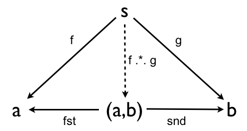
Suppose we have objects A and B in some category. Then their product (if it exists) is an object A×B, together with projections p1: A×B -> A, p2: A×B -> B, with the following universal property: whenever we have arrows f: S -> A and g: S -> B, then they can be factored through A×B to give an arrow f×g: S -> A×B, such that f = p1 . f×g, g = p2 . f×g.

(The definitions of product and coproduct are dual to one another - the diagrams are the same but with the directions of the arrows reversed.)

In the category Set, the product of sets A and B is their Cartesian product A×B. In the category Hask, of course, the product of types a and b is written (a,b), p1 is called fst, and p2 is called snd.

We can then define the required product map as:
(f .*. g) x = (f x, g x)

Then it should be clear that fst . (f .*. g) = f, and snd . (f .*. g) = g, as required.


Okay, so what do products look like in the category of lists (free monoids)? (Recall that in this category, the arrows are required to be monoid homomorphisms, meaning that f [] = [] and f (xs++ys) = f xs ++ f ys. It follows that we can express f = concatMap f', for some f'.)

Well, the obvious thing to try as the product is the Cartesian product ([a],[b]). Is the Cartesian product of two monoids a monoid? Well yes it is actually. We could give it a monoid structure as follows:

(as1, bs1) ++ (as2, bs2) = (as1++as2, bs1++bs2)
[] = ([],[])
This isn't valid Haskell code of course. It's just my shorthand way of expressing the following code from Data.Monoid:

instance Monoid [a] where
        mempty  = []
        mappend = (++)

instance (Monoid a, Monoid b) => Monoid (a,b) where
        mempty = (mempty, mempty)
        (a1,b1) `mappend` (a2,b2) =
                (a1 `mappend` a2, b1 `mappend` b2)

From these two instances, it follows that ([a],[b]) is a monoid, with monoid operations equivalent to those I gave above. (In particular, it's clear that the construction satisfies the monoid laws: associativity of ++, identity of [].)

But it feels like there's something unsatisfactory about this. Wouldn't it be better for the product of list types [a] and [b] to be another list type [x], for some type x?

Our first thought might be to try [(a.b)]. The product map would then need to be something like \ss -> zip (f ss) (g ss). However, we quickly see that this won't work: what if f ss and g ss are not the same length.

What else might work? Well, if you think of ([a],[b]) as some as on the left and some bs on the right, then the answer should spring to mind. Let's try [Either a b]. We can then define:

p1 xs = [x | Left x <- xs] -- this is doing a filter and a map at the same time
p2 xs = [x | Right x <- xs]
with the product map

f×g = \ss -> map Left (f ss) ++ map Right (g ss)

Then it is clear that p1 . f×g = f and p2 . f×g = g, as required.

What is the relationship between ([a],[b]) and [Either a b]? Well, ([a],[b]) looks a bit like a subset of [Either a b], via the injection i (as,bs) = map Left as ++ map Right bs. However, this injection is not a monoid homomorphism, since
i ([],[b1] ++ ([a1],[]) /= i ([],[b1]) ++ i ([a1],[])
So ([a],[b]) is not a submonoid of [Either a b].

On the other hand, there is a projection p :: [Either a b] -> ([a],[b]), p xs = (p1 xs, p2 xs). This is a monoid homomorphism, so ([a],[b]) is a quotient of [Either a b].


So which is the right answer? Which of ([a],[b]) and [Either a b] is really the product of [a] and [b]?

Well, it depends. It depends which category we think we're working in. If we're working in the category of monoids, then it is ([a],[b]). However, if we're working in the category of free monoids (lists), then it is [Either a b].

You see, ([a],[b]) is not a free monoid. What does this mean? Well, it basically means it's not a list. But how do we know that ([a],[b]) isn't equivalent to some list? And anyway, what does "free" mean in free monoid?

"Free" is a concept that can be applied to many algebraic theories, not just monoids. There is more than one way to define it.

An algebraic theory defines various constants and operations. In the case of monoids, there is one constant - which we may variously call [] or mempty or 0 or 1 - and one operation - ++ or mappend or + or *. Now, a given monoid may turn out to be generated by some subset of its elements - meaning that every element of the monoid can be equated with some expression in the generators, constants, and operations.

For example, the monoid of natural numbers is generated by the prime numbers: every natural number is equal to some expression in 1, *, and the prime numbers. The monoid [x] is generated by the singleton lists: every element of [x] is equal to some expression in [], ++, and the singleton lists. By a slight abuse of notation, we can say that [x] is generated by x - by identifying the singleton lists with the image of x under \x -> [x].

Then we say that a monoid is free on its generators if there are no relations among its elements other than those implied by the monoid laws. That is, no two expressions in the generators, constants, and operators are equal to one another, unless it is as a consequence of the monoid laws.

For example, suppose it happens that
(x ++ y) ++ z = x ++ (y ++ z)
That's okay, because it follows from the monoid laws. On the other hand, suppose that
x ++ y = y ++ x
This does not follow from the monoid laws (unless x = [] or y = []), so is a non-trivial relation. (Thus the natural numbers under multiplication are not a free monoid - because they're commutative.)

What about our type ([a],[b]) then? Well consider the following relations:

(as,[]) ++ ([],bs) = ([],bs) ++ (as,[])
(as1++as2,bs1) ++ ([],bs2) = (as1,bs1) ++ (as2,bs2) = (as1,[]) ++ (as2,bs1++bs2)
We have commutativity relations between the [a] and [b] parts of the product. Crucially, these relations are not implied by the monoid structure alone. So intuitively, we can see that ([a],[b]) is not free.

The "no relations" definition of free is the algebraic way to think about it. However, there is also a category theory way to define it. The basic idea is that if a monoid is free on its generators, then given any other monoid with the same generators, we can construct it as a homomorphic image of our free monoid, by "adding" the appropriate relations.

In order to express this properly, we're going to need to use some category theory, and specifically the concept of the forgetful functor. Recall that given any algebraic category, such as Mon (monoids), there is a forgetful functor U: Mon -> Set, which consists in simply forgetting the algebraic structure. U takes objects to their underlying sets, and arrows to the underlying functions. In Haskell, U: Mon -> Hask consists in forgetting that our objects (types) are monoids, and forgetting that our arrows (functions) are monoid homomorphisms. (As a consequence, U is syntactically invisible in Haskell. However, to properly understand the definition of free, we have to remember that it's there.)

Then, given an object x (the generators), a free monoid on x is a monoid y, together with a function i: x -> U y, such that whenever we have an object z in Mon and a function f': x -> U z, then we can lift it to a unique arrow f: y -> z, such that f' = Uf . i.

When we say that lists are free monoids, we mean specifically that (the type) [x] is free on (the type) x, via the function i = \x -> [x] (on values). This is free, because given any other monoid z, and function f' :: x -> z, then we can lift to a monoid homomorphism f :: [x] -> z, with f' = f . i. How? Well, the basic idea is to use concatMap. The type of concatMap is:
concatMap :: (a -> [b]) -> [a] -> [b]
So it's doing the lifting we want. However this isn't quite right, because this assumes that the target monoid z is a list. So we need this slight variant:

mconcatmap :: (Monoid z) => (x -> z) -> [x] -> z
mconcatmap f xs = mconcat (map f xs)
If we set f = mconcatmap f', then we will have

(f . i) x
= f (i x)
= f [x]
= mconcatmap f' [x]
= mconcat (map f' [x])
= mconcat [f' x]
= foldr mappend mempty [f' x]  -- definition of mconcat
= mappend mempty (f' x)  -- definition of foldr
= f' x  -- identity of mempty

Now, what would it mean for ([a],[b]) to be free? Well, first, what is it going to be free on? To be free on a and b is the same as being free on Either a b (the disjoint union of a and b). Then our function i is going to be

i (Left a) = ([a],[])
i (Right b) = ([],[b])
Then for ([a],[b]) to be free would mean that whenever we have a function f' :: Either a b -> z, with z a monoid, then we can lift it to a monoid homomorphism f : ([a],[b]) -> z, such that f' = f . i.

So can we?

Well, what if our target monoid z doesn't satisfy the a-b commutativity relations that we saw. That is, what if:
f' a1 `mappend` f' b1 /= f' b1 `mappend` f' a1 -- (A)
That would be a problem.

We are required to find an f such that f' = f . i.
We know that i a1 = ([a1],[]), i b1 = ([],[b1]). So we know that i a1 `mappend` i b1 = i b1 `mappend` i a1.
f is required to be a monoid homomorphism, so by definition:

f (i a1 `mappend` i b1) = f (i a1) `mappend` f (i b1)
f (i b1 `mappend` i a1) = f (i b1) `mappend` f (i a1)
But then since the two left hand sides are equal, then so are the two right hand sides, giving:
f (i a1) `mappend` f (i b1) = f (i b1) `mappend` f (i a1) -- (B)

But now we have a contradiction between (A) and (B), since f' = f . i.

So for a concrete counterexample, showing that ([a],[b]) is not free, all we need is a monoid z in which the a-b commutativity relations don't hold. Well that's easy: [Either a b]. Just take f' :: Either a b -> [Either a b], f' = \x -> [x]. Now try to find an f :: ([a],[b]) -> [Either a b], with f' = f . i.

The obvious f is f (as,bs) = map Left as ++ map Right bs.
But the problem is that this f isn't a monoid homomorphism:
f ( ([],[b1]) `mappend` ([a1],[]) ) /= f ([],[b1]) `mappend` f ([a1],[])


Notice the connection between the two definitions of free. It was because ([a],[b]) had non-trivial relations that we couldn't lift a function to a monoid homomorphism in some cases. The cases where we couldn't were where the target monoid z didn't satisfy the relations.

Okay, so sorry, that got a bit technical. To summarise, the product of [a], [b] in the category of lists / free monoids is [Either a b].


What about vector spaces? What is the product of Vect k a and Vect k b?

Well, similarly to lists, we can make (Vect k a, Vect k b) into a vector space, by defining
0 = (0,0)
(a1,b1) + (a2,b2) = (a1+a2,b1+b2)
k(a,b) = (ka,kb)

Exercise: Show that with these definitions, fst, snd and f .*. g are vector space morphisms (linear maps).

Alternatively, Vect k (Either a b) is of course a vector space. We can define:

p1 = linear p1' where
    p1' (Left a) = return a
    p1' (Right b) = zero

p2 = linear p2' where
    p2' (Left a) = zero
    p2' (Right b) = return b

prodf f g = linear fg' where
    fg' b = fmap Left (f (return b)) <+> fmap Right (g (return b))

In this case p1, p2, f×g are vector space morphisms by definition, since they were constructed using "linear". How do we know that they satisfy the product property? Well, this looks like a job for QuickCheck. The following code builds on the code we developed last time:

prop_Product (f',g',x) =
    f x == (p1 . fg) x &&
    g x == (p2 . fg) x
    where f = linfun f'
          g = linfun g'
          fg = prodf f g

newtype SBasis = S Int deriving (Eq,Ord,Show,Arbitrary)

prop_ProductQn (f,g,x) = prop_Product (f,g,x)
    where types = (f,g,x) :: (LinFun Q SBasis ABasis, LinFun Q SBasis BBasis, Vect Q SBasis)

> quickCheck prop_ProductQn
+++ OK, passed 100 tests.

As we did with lists, we can ask again, which is the correct definition of product, (Vect k a, Vect k b), or Vect k (Either a b)?

Well, in this case it turns out that they are equivalent to one another, via the mutually inverse isomorphisms

\(va,vb) -> fmap Left va <+> fmap Right vb
\v -> (p1 v, p2 v)
Unlike in the list case, these are both vector space morphisms (linear functions).

Why the difference? Why does it work out for vector spaces whereas it didn't for lists? Well, I think it's basically because vector spaces are commutative.

(It is also the case that vector spaces are always free on a basis. So since we have an obvious bijection between the bases of (Vect k a, Vect k b) and Vect k (Either a b), then we must have an isomorphism between the vector spaces.)


Now, we're left with a little puzzle. We have found that both the product and the coproduct of two vector spaces is Vect k (Either a b). So we still haven't figured out what Vect k (a,b) represents.

Coproducts of lists and free vector spaces

Recently we've been looking at vector spaces. We defined a type Vect k b, representing the free k-vector space over a type b - meaning, the vector space consisting of k-linear combinations of the inhabitants of b - so b is the basis. Like any good mathematical structure, vector spaces admit various new-from-old constructions. Last time I posed the puzzle, what do Vect k (Either a b) and Vect k (a,b) represent? As we're aiming for quantum algebra, I'm going to frame the answers in the language of category theory.

Suppose we have objects A and B in some category. Then their coproduct (if it exists) is an object A+B, together with injections i1: A -> A+B, i2: B -> A+B, with the following universal property: whenever we have arrows f: A -> T and g: B -> T, they can be factored through A+B to give an arrow f+g: A+B -> T, such that f = f+g . i1, g = f+g . i2.

Notice that this definition does not give us a construction for the coproduct. In any given category, it doesn't tell us how to construct the coproduct, or even if there is one. Even if we have a construction for the coproduct in one category, there is no guarantee that it, or something similar, will work in another related category.

In the category Set, the coproduct of sets A and B is their disjoint union. In order to see this, we can work in the category Hask of Haskell types. We can regard Hask as a subcategory of Set, by identifying a type with its set of inhabitants. If a and b are Haskell types / sets of inhabitants, then their disjoint union is Either a b. The elements of Either a b can be from either a or b (hence, from their union), and they are kept disjoint in the left and right parts of the union (so that for example Either a a contains two copies of a, not just one). The injections i1 and i2 are then the value constructors Left and Right. Given f :: a -> t, g :: b -> t, we define:

(f .+. g) (Left a) = f a
(f .+. g) (Right b) = g b
Then it should be clear that (f .+. g) . Left = f, and (f .+. g) . Right = g, as required

In a moment, we'll look at coproducts of vector spaces, but first, as a warmup, let's think about the coproducts in a simpler category: lists / free monoids. Recall that a monoid is an algebraic structure having an associative operation ++, and an identity for ++ called []. (That is [] ++ x = x = x ++ [].)

A monoid homomorphism is a function f :: [a] -> [b] such that f [] = [] and f (a1 ++ a2) = f a1 ++ f a2. With a little thought, you should be able to convince yourself that all monoid homomorphisms are of the form concatMap f', where f' :: a -> [b]. (Which is, incidentally, the same as saying that they are of the form (>>= f').) In the category of free monoids, the arrows are constrained to be monoid homomorphisms.

So for our coproduct, we are looking for an object satisfying the universal property shown in the following diagram:

Perhaps the first thing to try is the disjoint union: Either [a] [b]. This is the coproduct of [a] and [b] as sets, but is it also their coproduct as monoids? Well, let's see.

Hmm, firstly, it's not a list (doh!): so you can't apply ++ to it, and it doesn't have a []. However, before we give up on that, let's consider whether we're asking the right question. Perhaps we should only be requiring that Either [a] [b] is (or can be made to be) a Monoid instance. Is the disjoint union of two monoids a monoid? Suppose we try to define ++ for it:
Left a1 ++ Left a2 = Left (a1++a2)
Right b1 ++ Right b2 = Right (b1++b2)
But now we begin to see the problem. What are we going to do for Left as ++ Right bs? There's nothing sensible we can do, because our disjoint union Either [a] [b] does not allow mixed lists of as and bs.

However, this immediately suggests that we would be better off looking at [Either a b] - the free monoid over the disjoint union of a and b. This is a list - and it does allow us to form mixed lists of as and bs.

We can then set i1 = map Left, i2 = map Right, and these are list homomorphisms (they interact with [] and ++ in the required way). Then we can define:

h = concatMap h' where
    h' (Left a) = f' a
    h' (Right b) = g' b

So our suspicion is that [Either a b] is the coproduct, with h the required coproduct map.

Let's just check the coproduct conditions:
h . i1
= concatMap h' . map Left
= concatMap f'
= f
and similarly, h . i2 = g, as required.


Notice that the disjoint union Either [a] [b] is (isomorphic to) a subset of the free monoid [Either a b], via Left as -> map Left as; Right bs -> map Right bs. So we were thinking along the right lines in suggesting Either [a] [b]. The problem was that Either [a] [b] isn't a monoid, it's only a set. We can regard [Either a b] as the closure of Either [a] [b] under the monoid operations. [Either a b] is the smallest free monoid containing the disjoint union Either [a] [b] (modulo isomorphism of Haskell types).

(This is a bit hand-wavy. This idea of closure under algebraic operations makes sense in maths / set theory, but I'm not quite sure how best to express it in Haskell / type theory. If anyone has any suggestions, I'd be pleased to hear them.)

Okay, so what about a coproduct in the category of k-vector spaces. First, recall that the arrows in this category are linear maps f satisfying f (a+b) = f a + f b, f (k*a) = k * f a. Again, it should be obvious that a linear map is fully determined by its action on basis elements - so every linear map f :: Vect k a -> Vect k b can be expressed as linear f' where f' :: a -> Vect k b.

Recall that we defined linear f' last time - it's really just (>>= f'), but followed by reduction to normal form:
linear f v = nf $ v >>= f

Okay, so vector spaces of course have underlying sets, so we will expect the coproduct of Vect k a and Vect k b to contain the disjoint union Either (Vect k a) (Vect k b). As with lists though, we will have the problem that this is not closed under vector addition - we can't add an element of Vect k a to an element of Vect k b within this type.

So as before, let's try Vect k (Either a b). Then we can set i1 = fmap Left, i2 = fmap Right, and they are both linear maps by construction. (We don't need to call nf afterwards, since Left and Right are order-preserving.)

i1 = fmap Left
i2 = fmap Right
Then we can define the coproduct map (f+g) as follows:

coprodf f g = linear fg' where
    fg' (Left a) = f (return a)
    fg' (Right b) = g (return b)

We need to verify that this satisfies the coproduct conditions: f+g . i1 = f and f+g . i2 = g. It would be nice to test this using a QuickCheck property. In order to do that, we need a way to construct arbitrary linear maps. (This is not the same thing as arbitrary functions Vect k a -> Vect k b, so I don't think that I can use QuickCheck's Coarbitrary class - but the experts may know better.) Luckily, that is fairly straightforward: we can construct arbitrary lists [(a, Vect k b)], and then each pair (a,vb) can be interpreted as saying that the basis element a is taken to the vector vb.

type LinFun k a b = [(a, Vect k b)]

linfun :: (Eq a, Ord b, Num k) => LinFun k a b -> Vect k a -> Vect k b
linfun avbs = linear f where
    f a = case lookup a avbs of
          Just vb -> vb
          Nothing -> zero

With that preparation, here is a QuickCheck property that expresses the coproduct condition.

prop_Coproduct (f',g',a,b) =
    f a == (fg . i1) a &&
    g b == (fg . i2) b
    where f = linfun f'
          g = linfun g'
          fg = coprodf f g

That property can be used for any vector spaces. Let's define some particular vector spaces to do the test on.

newtype ABasis = A Int deriving (Eq,Ord,Show,Arbitrary) -- GeneralizedNewtypeDeriving
newtype BBasis = B Int deriving (Eq,Ord,Show,Arbitrary)
newtype TBasis = T Int deriving (Eq,Ord,Show,Arbitrary)

instance (Num k, Ord b, Arbitrary k, Arbitrary b) => Arbitrary (Vect k b) where
    arbitrary = do ts <- arbitrary :: Gen [(b, k)] -- ScopedTypeVariables
                   return $ nf $ V ts

(I should emphasize that not all vector space bases are newtypes around Int - we can have finite bases, or bases with other interesting internal structure, as we will see in later installments. For the purposes of this test however, I think this is sufficient.)

prop_CoproductQn (f,g,a,b) = prop_Coproduct (f,g,a,b)
    where types = (f,g,a,b) :: (LinFun Q ABasis TBasis, LinFun Q BBasis TBasis, Vect Q ABasis, Vect Q BBasis)

> quickCheck prop_CoproductQn
+++ OK, passed 100 tests.

So we do indeed have a coproduct on vector spaces. To summarise: The coproduct of free vector spaces is the free vector space on the coproduct (of the bases).

Next time, we'll look at products - where there might be a small surprise.

The free vector space on a type, part 2

Last time, I defined the free k-vector space over a type b:

data Vect k b = V [(b,k)]
Elements of Vect k b represent formal sums of scalar multiples of elements of b, where the scalars are taken from the field k. (For example, V [(E1,5),(E3,2)] represents the formal sum 5E1+2E3.) Thus b is the basis for the vector space.

We saw that there is a functor (in the mathematical sense) from the category Hask (of Haskell types and functions) to the category k-Vect (of k-vector spaces and k-linear maps). In maths, we would usually represent a functor by a capital letter, eg F, and apply it to objects and arrows by prefixing. For example, if a, b are objects in the source category, then the image objects in the target category would be called F a and F b. If f :: a -> b is an arrow in the source category, then the image arrow in the target category would be called F f.

Haskell allows us to declare a type constructor as a Functor instance, and give it an implementation of fmap. This corresponds to describing a functor (in the mathematical sense), but with a different naming convention. In our case, we declared the type constructor (Vect k) as a Functor instance. So the functor's action on objects is called (Vect k) - given any object b in Hask (ie a Haskell type), we can apply (Vect k) to get an object Vect k b in k-Vect (ie a k-vector space). However, the functor's action on arrows is called fmap - given any arrow f :: a -> b in Hask (ie a Haskell function), we can apply fmap to get an arrow fmap f :: Vect k a -> Vect k b in k-Vect (ie a k-linear map).

Haskell allows us to declare only type constructors as functors. In maths, there are many functors which are not of this form. For example, the simplest is the forgetful functor. Given any algebraic category A, we have the forgetful functor A -> Set, which simply forgets the algebraic structure. The forgetful functor takes the objects of A to their underlying sets, and the arrows of A to the underlying functions.

For example, in our case, the forgetful functor k-Vect -> Hask consists in forgetting that the objects Vect k b are vector spaces (with addition, scalar multiplication etc defined), and considering them just as Haskell types; and forgetting that the arrows Vect k a -> Vect k b are linear maps, and considering them just as Haskell functions.

(Notice that when working in Haskell, the category Hask acts as a kind of stand-in for the category Set. If we identify a type with its inhabitants (which form a set), then Hask is something like the computable subcategory of Set.)


So we actually have functors going both ways. We have the free functor F: Hask -> k-Vect - which takes types and functions to free k-vector spaces and linear maps. And we have the forgetful functor G: k-Vect -> Hask - which takes free k-vector spaces and linear maps, and just forgets their algebraic structure, so that they're just types and functions again.

Note that these two functors are not mutual inverses. (G . F) is not the identity on Hask - indeed it takes b to Vect k b, both considered as objects in Hask (and similarly with arrows). The two functors are however adjoint. (I'm not going to explain what this means, but see Wikipedia, or most books on category theory.)

Whenever we have an adjunction, then in fact we also have a monad. Here's the definition for our case:

instance Num k => Monad (Vect k) where
    return a = V [(a,1)]
    V ts >>= f = V $ concat [ [(b,y*x) | let V us = f a, (b,y) <- us] | (a,x) <- ts]

This monad is most easily understood using the monad as container analogy. A free k-vector space over b is just a container of elements of b. Okay, so it's a slightly funny sort of container. It most resembles a multiset or bag - an unordered container in which you can have more than one of each element. However, free k-vector spaces go further. A free Q-vector space is a container in which we're allowed to have fractional or negative amounts of each basis element, such as 1/2 e1 - 3 e2. In a free C-vector space, we're even allowed imaginary amounts of each element, such as i e3.

These oddities aside though, free k-vector spaces are monads in much the same way as any other container. For example, let's compare them to the list monad.
- For a container monad, return means "put into the container". For List, return a is [a]. For k-Vect, return a is 1 a (where 1 is the scalar 1 in our field k).
- For container monads, it's most natural to look next at the join operation, which combines a container of containers into a single container. For List, join = concat. For k-Vect, join combines a linear combination of linear combinations into a single linear combination (in the obvious way).
- Finally there is bind or (>>=). bind can be defined in terms of join and fmap:
x >>= f = join ((fmap f) x)
For lists, bind is basically concatMap. For k-Vect, bind corresponds to extending a function on basis elements to a function on vectors "by linearity". That is, if f :: a -> Vect k b, then (>>= f) :: Vect k a -> Vect k b is defined (in effect, by structural induction) so as to be linear, by saying that (>>= f) 0 = 0, (>>= f) (k a) = k (f a), (>>= f) (a + b) = f a + f b.

So k-Vect is like just a strange sort of list. Think of them as distant cousins. Incidentally, this is not only because they're both containers (if you believed my story about k-Vect being a container). There's another reason: Both the List and k-Vect monads arise from free-forgetful adjunctions. In the case of lists, the list datatype is the free monoid, and the list monad arises from the free-forgetful adjunction for monoids.

That's most of what I wanted to say for now. However, there's one small detail to add. Last time we defined a normal form for elements of Vect k b, in which the basis elements are in order, without repeats, and none of the scalars are zero. In order to calculate this normal form, we require an Ord instance for b. Unfortunately, Haskell doesn't let us specify that when defining the Monad instance for (Vect k). So whenever we use (>>=), we should call nf afterwards, to put the result in normal form.

For this reason, we define a convenience function:

linear :: (Ord b, Num k) => (a -> Vect k b) -> Vect k a -> Vect k b
linear f v = nf $ v >>= f
Given f :: a -> Vect k b, linear f :: Vect k a -> Vect k b is the extension of f from basis elements to vectors "by linearity". Hence, linear f is guaranteed to be linear, by construction. We can confirm this on an example using the QuickCheck properties we defined last time.

> let f (E 1) = e1; f (E 2) = e1 <+> e2; f _ = zero
> (linear f) (e1 <+> e2)
2e1+e2
> quickCheck (prop_LinearQn (linear f))
+++ OK, passed 100 tests.

Acknowledgement: I'm partially retreading in Dan Piponi's steps here. He first described the free vector space monad here. When I come to discuss the connection between quantum algebra and knot theory, I'll be revisiting some more material that Dan sketched out here.

Exercise for next time: What does Vect k (Either a b) represent? What does Vect k (a,b) represent?

The free vector space on a type, part 1

As I mentioned last time, I want to spend the next few posts talking about quantum algebra. Well, we've got to start somewhere, so let's start with vector spaces.

You probably know what a vector space is. It's what is sounds like: a space of vectors, that you can add together, or multiply by scalars (that is, real numbers, or more generally, elements of some field k). Here's the official definition:
An additive (or Abelian) group is a set with a binary operation called addition, such that
- addition is associative: x+(y+z) = (x+y)+z
- addition is commutative: x+y = y+x
- there is an additive identity: x+0 = x = 0+x
- there are additive inverses: x+(-x) = 0 = (-x)+x
A vector space over a field k is an additive group V, together with an operation k * V -> V called scalar multiplication, such that:
- scalar multiplication distributes over vector addition: a(x+y) = ax+ay
- scalar multiplication distributes over scalar addition: (a+b)x = ax+bx
- associativity: (ab)x = a(bx)
- unit: 1a = a

There are some obvious examples:
- R^2 is a 2-dimensional vector space over the reals R, R^3 is a 3-dimensional vector space. (I'm not going to define dimension quite yet, but hopefully it's intuitively obvious what it means.)
- R^n is an R-vector space for any n.
- Indeed, k^n is a k-vector space for any field k.

Some slightly more interesting examples:
- C is a 2-dimensional vector space over R. (The reason it's more interesting is that of course C possesses additional algebraic structure, beyond the vector space structure.)
- 2*2 matrices over k form a 4-dimensional k-vector space.
- Polynomials in X with coefficients in k form an (infinite dimensional) k-vector space.


If we wanted to code the above definition into Haskell, probably the first idea that would come to mind would be to use type classes:

class AddGrp a where
    add :: a -> a -> a
    zero :: a
    neg :: a -> a -- additive inverse

class (Field k, AddGrp v) => VecSp k v where
    smult :: k -> v -> v -- scalar multiplication

(Type classes similar to these are defined are in the vector-space package.)


For most vector spaces that one encounters in "real life", there is some set of elements, usually obvious, which form a "basis" for the vector space, meaning that all elements can be expressed as linear combinations of basis elements. For example, in R^3, the obvious basis is {(0,0,1), (0,1,0), (1,0,0)}. Any element (x,y,z) of R^3 can be expressed as the linear combination x(1,0,0)+y(0,1,0)+z(0,0,1).

(Mathematicians would want to stress that there are other bases for R^3 that would serve equally well, and indeed, that a significant part of the theory of vector spaces can go through without even talking about bases. However, for our purposes - we want to write code to calculate in vector spaces - then working with a basis is natural.)


Okay, so we want a way to build a vector space from a basis. (More specifically, a k-vector space, for some given field k.) What sorts of things shall we allow as our basis? Well, why not just allow any type, whatsoever:

module Math.Algebras.VectorSpace where

import qualified Data.List as L

data Vect k b = V [(b,k)] deriving (Eq,Ord)

This says that a k-vector space over basis b consists of a linear combination of elements of b. (So the [(b,k)] is to be thought of as a sum, with each (b,k) pair representing a basis element in b multiplied by a scalar coefficient in k.)

For example, we can define the "boring basis" type, which just consists of numbered basis elements:

newtype EBasis = E Int deriving (Eq,Ord)

instance Show EBasis where show (E i) = "e" ++ show i

e i = return (E i) -- don't worry about what "return" is doing here for the moment
e1 = e 1
e2 = e 2
e3 = e 3

Then a typical element of Vect Double EBasis is:

> :load Math.Algebras.VectorSpace
> V [(E 1, 0.5), (E 3, 0.7)]
0.5e1+0.7e3

So of course, the Show instances for EBasis (see above), and Vect k b (not shown) are coming into play here.

How do we know that this is a vector space? Well actually, it's not yet, because we haven't defined the addition and scalar multiplication operations on it. So, without further ado:

infixr 7 *>
infixl 6 <+>

-- |The zero vector
zero :: Vect k b
zero = V []

-- |Addition of vectors
add :: (Ord b, Num k) => Vect k b -> Vect k b -> Vect k b
add (V ts) (V us) = V $ addmerge ts us

-- |Addition of vectors (same as add)
(<+>) :: (Ord b, Num k) => Vect k b -> Vect k b -> Vect k b
(<+>) = add

addmerge ((a,x):ts) ((b,y):us) =
    case compare a b of
    LT -> (a,x) : addmerge ts ((b,y):us)
    EQ -> if x+y == 0 then addmerge ts us else (a,x+y) : addmerge ts us
    GT -> (b,y) : addmerge ((a,x):ts) us
addmerge ts [] = ts
addmerge [] us = us

-- |Negation of vector
neg :: (Num k) => Vect k b -> Vect k b
neg (V ts) = V $ map (\(b,x) -> (b,-x)) ts

-- |Scalar multiplication (on the left)
smultL :: (Num k) => k -> Vect k b -> Vect k b
smultL 0 _ = zero -- V []
smultL k (V ts) = V [(ei,k*xi) | (ei,xi) <- ts]

-- |Same as smultL. Mnemonic is "multiply through (from the left)"
(*>) :: (Num k) => k -> Vect k b -> Vect k b
(*>) = smultL

A few things to mention:
- First, note that we required a Num instance for k. Strictly speaking, as we stated that k is a field, then we should have required a Fractional instance. However, on occasion we are going to break the rules slightly.
- Second, note that for addition, we required an Ord instance for b. We could have defined addition using (++) to concatenate linear combinations - however, the problem with that is that it wouldn't then easily follow that e1+e3 = e3+e1, or that e1+e1 = 2e1. By requiring an Ord instance, we can guarantee that there is a unique normal form in which to express any vector - namely, list the basis elements in order, combine duplicates, remove zero coefficients.
- Finally, note that I didn't define Vect k b as an instance of a vector space type class. That's just because I didn't yet see a reason to.

It will turn out to be useful to have a function that can take an arbitrary element of Vect k b and return a vector in normal form:

-- |Convert an element of Vect k b into normal form. Normal form consists in having the basis elements in ascending order,
-- with no duplicates, and all coefficients non-zero
nf :: (Ord b, Num k) => Vect k b -> Vect k b
nf (V ts) = V $ nf' $ L.sortBy compareFst ts where
    nf' ((b1,x1):(b2,x2):ts) =
        case compare b1 b2 of
        LT -> if x1 == 0 then nf' ((b2,x2):ts) else (b1,x1) : nf' ((b2,x2):ts)
        EQ -> if x1+x2 == 0 then nf' ts else nf' ((b1,x1+x2):ts)
        GT -> error "nf': not pre-sorted"
    nf' [(b,x)] = if x == 0 then [] else [(b,x)]
    nf' [] = []
    compareFst (b1,x1) (b2,x2) = compare b1 b2

Okay, so we ought to check that the Vect k b is a vector space. Let's write some QuickCheck properties:

prop_AddGrp (x,y,z) =
    x <+> (y <+> z) == (x <+> y) <+> z && -- associativity
    x <+> y == y <+> x                 && -- commutativity
    x <+> zero == x                    && -- identity
    x <+> neg x == zero                   -- inverse

prop_VecSp (a,b,x,y,z) =
    prop_AddGrp (x,y,z) &&
    a *> (x <+> y) == a *> x <+> a *> y && -- distributivity through vectors
    (a+b) *> x == a *> x <+> b *> x     && -- distributivity through scalars
    (a*b) *> x == a *> (b *> x)         && -- associativity
    1 *> x == x                            -- unit

instance Arbitrary EBasis where
    arbitrary = do n <- arbitrary :: Gen Int
                   return (E n)

instance Arbitrary Q where
    arbitrary = do n <- arbitrary :: Gen Integer
                   d <- arbitrary :: Gen Integer
                   return (if d == 0 then fromInteger n else fromInteger n / fromInteger d)

instance Arbitrary (Vect Q EBasis) where
    arbitrary = do ts <- arbitrary :: Gen [(EBasis, Q)]
                   return $ nf $ V ts

prop_VecSpQn (a,b,x,y,z) = prop_VecSp (a,b,x,y,z)
    where types = (a,b,x,y,z) :: (Q, Q, Vect Q EBasis, Vect Q EBasis, Vect Q EBasis)

> quickCheck prop_VecSpQn
+++ OK, passed 100 tests.

(I'm using Q instead of R as my field in order to avoid false negatives caused by the fact that arithmetic in Double is not exact.)

So it looks like Vect k b is indeed a vector space. In category theory, it is called the free k-vector space over b. "Free" here means that there are no relations among the basis elements: it will never turn out, for example, that e1 = e2+e3.


Vector spaces of course form a category, specifically an algebraic category (there are other types, as we'll see in due course). The objects in the category are the vector spaces. The arrows or morphisms in the category are the functions between vector spaces which "commute" with the algebraic structure. Specifically, they are the functions f such that:
- f(x+y) = f(x)+f(y)
- f(0) = 0
- f(-x) = -f(x)
- f(a.x) = a.f(x)

Such a function is called linear, the idea being that it preserves lines. This is because it follows from the the conditions that f(a.x+b.y) = a.f(x)+b.f(y) .

We can write a QuickCheck property to check whether a given function is linear:

prop_Linear f (a,x,y) =
    f (x <+> y) == f x <+> f y &&
    f zero == zero             &&
    f (neg x) == neg (f x)     &&
    f (a *> x) == a *> f x

prop_LinearQn f (a,x,y) = prop_Linear f (a,x,y)
    where types = (a,x,y) :: (Q, Vect Q EBasis, Vect Q EBasis)

For example:

> quickCheck (prop_LinearQn (2 *>))
+++ OK, passed 100 tests.

We won't need to use this quite yet, but it's handy to have around.


Now, in category theory we have the concept of a functor, which is a map from one category to another, which commutes with the category structure. Specifically, a functor F consists of a map from the objects of one category to the objects of the other, and from the arrows of one category to the arrows of the other, satisfying:
- F(id_A) = id_F(A)
- F(f . g) = F(f) . F(g) (where dot denotes function composition)

How does this relate to the Functor type class in Haskell? Well, the Haskell type class enables us to declare that a /type constructor/ is a functor. For example, (Vect k) is a type constructor, which acts on a type b to construct another type Vect k b. (Vect k) is indeed a functor, witness the following declaration:

instance Functor (Vect k) where
    fmap f (V ts) = V [(f b, x) | (b,x) <- ts]

This says that if we have a function f on our basis elements, then we can lift it to a function on linear combinations of basis elements in the obvious way.

In mathematics, we would think of the free vector space construction as a functor from Set (the category of sets) to k-Vect (the category of k-vector spaces). In Haskell, we need to think of the (Vect k) construction slightly differently. It operates on types, rather than sets, so the source category is Hask, the category of Haskell types.

What is the relationship between Hask and Set? Well, if we identify a type with the set of values which inhabit it, then we can regard Hask as a subcategory of Set, consisting of those sets and functions which can be represented in Haskell. (That would imply for example that we are restricted to computable functions.)

So (Vect k) is a functor from Hask to the subcategory of k-Vect consisting of vector spaces over sets/types in Hask.

So just to spell it out, the (Vect k) functor:
- Takes an object b in Hask/Set - ie a type, or its set of inhabitants - to an object Vect k b in k-Vect
- Takes an arrow f in Hask (ie a function f :: a -> b), to an arrow (fmap f) :: Vect k a -> Vect k b in k-Vect.

Now, there's just one small fly in the ointment. In order to get equality of vectors to work out right, we wanted to insist that they were expressed in normal form, which meant we needed an Ord instance for b. However, in the Functor instance for (Vect k), Haskell doesn't let us express this constraint, and our fmap is unable to use the Ord instance for b. What this means is that fmap f might return a vector which is not in normal form - so we need to remember to call nf afterwards. For example:

newtype FBasis = F Int deriving (Eq,Ord)

instance Show FBasis where show (F i) = "f" ++ show i

> let f = \(E i) -> F (10 - div i 2)
> let f' = fmap f :: Vect Q EBasis -> Vect Q FBasis
> f' (e1 <+> 2 *> e2 <+> e3)
f10+2f9+f9
> let f'' = nf . fmap f :: Vect Q EBasis -> Vect Q FBasis
> f'' (e1 <+> 2 *> e2 <+> e3)
3f9+f10

So it might be fairer to say that it is the combination of nf and fmap that forms the functor on arrows.

The definition of a functor requires that the target arrow is an arrow in the target category. In this case, the requirement is that it is a linear function, rather than just any function between vector spaces. So let's just check:

> quickCheck (prop_LinearQn f'')
+++ OK, passed 100 tests.

That's enough for now - more next time.

New modules - Quantum Algebra

I've put up a new version of HaskellForMaths on Hackage, v0.3.1. It's quite a significant update, with more than a dozen new modules, plus improved documentation of several existing modules. I wrote the new modules in the course of reading Kassel's Quantum Groups. The modules are about algebras, coalgebras, bialgebras, Hopf algebras, tensor categories and quantum algebra.

The new modules fall into two groups:

• Math.Algebras.* - Modules about algebras (and co-, bi- and Hopf algebras) in general
• Math.QuantumAlgebra.* - Modules specifically about quantum algebra

In (slightly) more detail, here are the modules:

• Math.Algebras.VectorSpace - defines a type for the free k-vector space over a basis set b 
• Math.Algebras.TensorProduct  - defines tensor product of two vector spaces
• Math.Algebras.Structures - defines a number of additional algebraic structures that can be given to vector spaces: algebra, coalgebra, bialgebra, Hopf algebra, module, comodule
• Math.Algebras.Quaternions - a simple example of an algebra
• Math.Algebras.Matrix - the 2*2 matrices - another simple example of an algebra
• Math.Algebras.Commutative - commutative polynomials (such as x^2+3yz) - another algebra
• Math.Algebras.NonCommutative - non-commutative polynomials (where xy /= yx) - another algebra
• Math.Algebras.GroupAlgebra - a key example of a Hopf algebra
• Math.Algebras.AffinePlane - the affine plane and its symmetries - more Hopf algebras, preparing for the quantum plane
• Math.Algebras.TensorAlgebra
• Math.Algebras.LaurentPoly - we use Laurent polynomials in q (that is, polynomials in q and q^-1) as our quantum scalars

• Math.QuantumAlgebra.QuantumPlane - the quantum plane and its symmetries, as examples of non-commutative, non-cocommutative Hopf algebras
• Math.QuantumAlgebra.TensorCategory
• Math.QuantumAlgebra.Tangle - The tangle category (which includes knots, links and braids as subcategories), and some representations (from which we derive knot invariants)
• Math.QuantumAlgebra.OrientedTangle

The following diagram is something like a dependency diagram, with "above" meaning "depends on".

Each layer depends on the layers beneath it. There are also a few dependencies within layers, that I've hinted at by proximity.

Some of these modules overlap somewhat in content with other modules that already exist in HaskellForMaths. In particular, there are already modules for commutative algebra, non-commutative algebra, and knot theory. For the moment, those existing modules still offer some features not offered by the new modules (for example, calculation of Groebner bases).

For the next little while in this blog, I want to start going through these new modules, and investigating quantum algebra. I should emphasize that this is still work in progress. For example, I'm intending to add modules for quantum enveloping algebras - but I have some reading to do first.

(Oh, and I know that I did previously promise to look at finite simple groups, and Coxeter groups, in this blog. I'll probably still come back to those at some point.)

Word length in the Symmetric group

Previously on this blog, we saw how to think about groups abstractly via group presentations, where a group is given as a set of generators satisfying specified relations. Last time, we saw that questions about the length of reduced words in such a presentation can be visualised as questions about the length of paths in the Cayley graph of the group (relative to the generators).

This time, I want to focus on just one family of groups - the symmetric groups Sn, as generated by the adjacent transpositions {si = (i i+1)}. Here's the Haskell code defining this presentation of Sn:

newtype SGen = S Int deriving (Eq,Ord)

instance Show SGen where
    show (S i) = "s" ++ show i

_S n = (gs, r ++ s ++ t) where
    gs = map S [1..n-1]
    r = [([S i, S i],[]) | i <- [1..n-1]]
    s = [(concat $ replicate 3 [S i, S (i+1)],[]) | i <- [1..n-2]]
    t = [([S i, S j, S i, S j],[]) | i <- [1..n-1], j <- [i+2..n-1]]

The three sets of relations say: each generator si squares to the identity; if i, j are not adjacent, then si and sj commute; if i, j are adjacent, then (si*sj)^3 is the identity.

Here is the Cayley graph for S4 under this presentation:

The vertices are labeled with the reduced words in the generators si. How can we find out which permutations these correspond to? Well, that's easy:

fromTranspositions ts = product $ map (\(S i) -> p [[i,i+1]]) ts
For example:

> :load Math.Algebra.Group.CayleyGraph
> fromTranspositions [S 1, S 2, S 1, S 3, S 2, S 1]
[[1,4],[2,3]]
This is the permutation that reverses the list [1..4]

> map (.^ it) [1..4]
[4,3,2,1]
What about the other way round? Suppose we are given a permutation in Sn. How do we find its expression as a product of the transpositions si? Well the answer is (roughly): use bubblesort!

Here's bubblesort in Haskell:

bubblesort [] = []
bubblesort xs = bubblesort' [] xs where
    bubblesort' ls (r1:r2:rs) = if r1 <= r2 then bubblesort' (r1:ls) (r2:rs) else bubblesort' (r2:ls) (r1:rs)
    bubblesort' ls [r] = bubblesort (reverse ls) ++ [r]

So we sweep through the list from front to back, swapping any pairs that we find out of order - and then repeat. At the end of each sweep, we're guaranteed that the last element (in sort order) has reached the end of the list - so for the next sweep, we can leave it at the end and only sweep through the earlier elements. Hence the list we're sweeping through is one element shorter each time, so we're guaranteed to terminate. (We could terminate early, the first time a sweep makes no swaps - but I haven't coded that.)

Just to prove that the code works:

> bubblesort [2,3,1]
[1,2,3]
How does this help for turning a permutation into a sequence of transpositions? Well it's simple - every time we swap two elements, we are performing a transposition - so just record which swaps we perform. So here's a modified version of the above code, which records the swaps:

-- given a permutation of [1..n] (as a list), return the transpositions which led to it
toTrans [] = []
toTrans xs = toTrans' 1 [] [] xs where
    toTrans' i ts ls (r1:r2:rs) =
        if r1 <= r2
        then toTrans' (i+1) ts (r1:ls) (r2:rs)         -- no swap needed
        else toTrans' (i+1) (S i : ts) (r2:ls) (r1:rs) -- swap needed
    toTrans' i ts ls [r] = toTrans (reverse ls) ++ ts

Notice that the ts are returned in reverse to the order that they were used. This is because we are using them to undo the permutation - so we are performing the inverse of the permutation we are trying to find. Since each generator is its own inverse, we can recover the permutation we are after simply by reversing. In the code, we reverse as we go along.

For example:

> toTrans [2,3,1]
[s1,s2]
> toTrans [4,3,2,1]
[s1,s2,s1,s3,s2,s1]
Now, there's only one problem. As you can see, this code takes as input a rearrangement of [1..n]. This is a permutation, yes, but considered passively. Whereas in this blog we have been more accustomed to thinking of permutations actively, as something a bit like a function, which has an action on a graph, or other combinatorial structure, or if you like, just on the set [1..n]. In other words, our Permutation type represents the action itself, not the outcome of the action. (Recall that the implementation uses a Data.Map of (from,to) pairs.)

But of course it's easy to convert from one viewpoint to the other. So here's the code to take a permutation in cycle notation and turn it into a sequence of transpositions:

-- given a permutation action on [1..n], factor it into transpositions
toTranspositions 1 = []
toTranspositions g = toTrans [i .^ (g^-1) | i <- [1..n] ] where
    n = maximum $ supp g

For example:

> toTranspositions $ p [[1,4],[2,3]]
[s1,s2,s1,s3,s2,s1]
Why does the code have [i .^ (g^-1) | i <- [1..n]], rather than [i .^ g | i <- [1..n]]?
Well, suppose i .^ g = j. This says that g moves i to the j position. But we want to know what ends up in the i position. Suppose that j .^ g = i, for some j. Applying g^-1 to both sides, we see that j = i .^ (g^-1).


Okay, so given a permutation, in either form, we can reconstruct it as a reduced word in the generators.

We saw last time that the length of a reduced word is also the length of the shortest path from 1 to the element in the Cayley graph. Distance in the Cayley graph is a metric on the group, so the length of a reduced word tells us "how far" the element is from being the identity.

If it's only this distance that we're interested in, then there is a more direct way to work it out. Given a permutation g of [1..n], then an inversion is a pair (i,j) with i < j but i .^ g > j .^ g. In Haskell:

inversions g = [(i,j) | i <- [1..n], j <- [i+1..n], i < j, i .^ g > j .^ g]
    where n = maximum $ supp g

For example:

> inversions $ fromList [1,4,3,2]
[(2,3),(2,4),(3,4)]
With a little thought, you should be able to convince yourself that the number of inversions is equal to the length of the reduced word for g - because each swap that we perform during bubblesort corrects exactly one inversion.

Okay, so this is all very nice, but what use is it? Well, of course, maths doesn't have to be useful, any more than any other aesthetic pursuit. However, as it happens, in this case it is.

In statistics, the Kendall tau test gives an indicator of the correlation between two measured quantities (for example, the height and weight of the test subjects). Suppose that we are given a list of pairs (eg (height,weight) pairs), and we want to know how strongly correlated the first and second quantities are.

Ok, so what we do is, we rank the first quantities from lowest to highest, and replace each quantity by its rank (a number from 1 to n). We do the same for the second quantities. So we end up with a list of pairs of numbers from 1 to n. Now, we sort the list on the first element, and then count the number of inversions in the second element.

For example, suppose our original list was [(1.55m, 60kg), (1.8m, 80kg), (1.5m, 70kg), (1.6m, 72kg)]. Converting to ranks, we get [(2nd,1st),(4th,4th),(1st,2nd),(3rd,3rd)]. Sorting on fst, we get [(1,2),(2,1),(3,3),(4,4)]. Looking at snd, we see that we have just one inversion. The idea is that the fewer inversions we have, the better correlated the two quantities. (Of course in reality there's a bit more to it than that - to convert the number of inversions into a probability, we need to know the distribution of word lengths for Sn, where n is the number of pairs of test data that we have.)

So you can think of the Kendall tau test as saying: What permutation has been applied in moving from the first quantities (the heights) to the second quantities (the weights)? How far is that permutation from the identity (on the Cayley graph)? What proportion of all permutations (in Sn) lie at that distance or less from the identity? (Even more concretely, we can imagine colouring in successive shells of the Cayley graph, working out from the identity, until we hit the given permutation, and then asking what proportion of the "surface" of the graph has been coloured.)