CHAs II: The Hopf Algebra SSym of Permutations

Last time we looked at YSym, the (dual of the) Loday-Ronco Hopf algebra of binary trees. This time I want to look at SSym, the Malvenuto-Reutenauer Hopf algebra of permutations. (In due course we'll see that YSym and SSym are quite closely related.)

The fundamental basis for SSym is (indexed by) the permutations of [1..n] for n <- [0..]. As usual, we work in the free vector space over this basis. Hence a typical element of SSym might be something like [1,3,2] + 2 [4,1,3,2]. Here's some code:

newtype SSymF = SSymF [Int] deriving (Eq)

instance Ord SSymF where
    compare (SSymF xs) (SSymF ys) = compare (length xs, xs) (length ys, ys)

instance Show SSymF where
    show (SSymF xs) = "F " ++ show xs

ssymF :: [Int] -> Vect Q SSymF
ssymF xs | L.sort xs == [1..n] = return (SSymF xs)
         | otherwise = error "Not a permutation of [1..n]"
         where n = length xs

(The "F" in SSymF stands for fundamental basis: we may have cause to look at other bases in due course.)

Let's try it out:

$ cabal update
$ cabal install HaskellForMaths
$ ghci
> :m Math.Algebras.Structures Math.Combinatorics.CombinatorialHopfAlgebra
> ssymF [1,3,2] + 2 * ssymF [4,1,3,2]
F [1,3,2]+2F [4,1,3,2]

Ok, so how can we define an algebra structure on this basis? How can we multiply permutations? (We want to consider permutations as combinatorial rather than algebraic objects here. So no, the answer isn't the group algebra.) One possibility would be to use the following shifted concatenation operation:

shiftedConcat (SSymF xs) (SSymF ys) = let k = length xs in SSymF (xs ++ map (+k) ys)

For example:

> shiftedConcat (SSymF [1,2]) (SSymF [2,1,3])
F [1,2,4,3,5]

This has the required properties. It's associative:

> quickCheck (\x y z -> shiftedConcat (shiftedConcat x y) z == shiftedConcat x (shiftedConcat y z))
+++ OK, passed 100 tests.

And it's pretty obvious that the empty permutation, SSymF [], is a left and right identity. Hence we could form a monoid algebra using this operation.

However, for the Hopf algebra we're going to look at, we will use a slightly more complicated multiplication. We will retain the idea of shifting the second permutation, so that the two lists are disjoint. However, instead of just concatenating them, we will form the sum of all possible "shuffles" of the two lists. Here's the shuffle code:

shuffles (x:xs) (y:ys) = map (x:) (shuffles xs (y:ys)) ++ map (y:) (shuffles (x:xs) ys)
shuffles xs [] = [xs]
shuffles [] ys = [ys]

So shuffles takes two input "decks of cards", and it outputs all possible ways that they can be shuffled together, while preserving the order between cards from the same deck. For example:

> shuffles [1,2] [3,4,5]
[[1,2,3,4,5],[1,3,2,4,5],[1,3,4,2,5],[1,3,4,5,2],[3,1,2,4,5],[3,1,4,2,5],[3,1,4,5,2],[3,4,1,2,5],[3,4,1,5,2],[3,4,5,1,2]]

Notice how in each of the output shuffles, we have 1 before 2, and 3 before 4 before 5. This enables us to define an algebra structure on permutations as follows:

instance (Eq k, Num k) => Algebra k SSymF where
    unit x = x *> return (SSymF [])
    mult = linear mult'
        where mult' (SSymF xs, SSymF ys) =
                  let k = length xs
                  in sumv [return (SSymF zs) | zs <- shuffles xs (map (+k) ys)]

For example:

> ssymF [1,2] * ssymF [2,1,3]
F [1,2,4,3,5]+F [1,4,2,3,5]+F [1,4,3,2,5]+F [1,4,3,5,2]+F [4,1,2,3,5]+F [4,1,3,2,5]+F [4,1,3,5,2]+F [4,3,1,2,5]+F [4,3,1,5,2]+F [4,3,5,1,2]

It's clear that ssymF [] is indeed a left and right unit for this multiplication. It's also fairly clear that this multiplication is associative (because both shifting and shuffling are). Let's just check:

> quickCheck (prop_Algebra :: (Q, Vect Q SSymF, Vect Q SSymF, Vect Q SSymF) -> Bool)
+++ OK, passed 100 tests.

(The test code isn't exposed in the package, so you'll have to dig around in the source if you want to try this. It takes a minute or two, because every time we multiply we end up with lots of terms.)


What about a coalgebra structure? As I mentioned last time, in a combinatorial Hopf algebra, the comultiplication is usually a sum of the different ways to take apart our combinatorial object into two parts. In this case, we take a permutation apart by "deconcatenating" it (considered as a list) into two pieces. This is like cutting a deck of cards:

deconcatenations xs = zip (inits xs) (tails xs)

For example:

> deconcatenations [2,3,4,1]
[([],[2,3,4,1]),([2],[3,4,1]),([2,3],[4,1]),([2,3,4],[1]),([2,3,4,1],[])]

However, most of those parts are no longer permutations of [1..n] (for any n), because they are missing some numbers. In order to get back to permutations, we need to "flatten" each part:

flatten xs = let mapping = zip (L.sort xs) [1..]
        in [y | x <- xs, let Just y = lookup x mapping]

For example:

> flatten [3,4,1]
[2,3,1]

Putting the deconcatenation and flattening together we get the following coalgebra definition:

instance (Eq k, Num k) => Coalgebra k SSymF where
    counit = unwrap . linear counit' where counit' (SSymF xs) = if null xs then 1 else 0
    comult = linear comult'
        where comult' (SSymF xs) = sumv [return (SSymF (flatten us), SSymF (flatten vs))
                                        | (us, vs) <- deconcatenations xs]

For example:

> comult $ ssymF [2,3,4,1]
(F [],F [2,3,4,1])+(F [1],F [2,3,1])+(F [1,2],F [2,1])+(F [1,2,3],F [1])+(F [2,3,4,1],F [])

(Recall that the result should be read as F[]⊗F[2,3,4,1] + F[1]⊗F[2,3,1] + ...)

It's fairly clear that this comultiplication is coassociative. The counit properties are equally straightforward. Hence:

> quickCheck (prop_Coalgebra :: Vect Q SSymF -> Bool)
+++ OK, passed 100 tests.

Is it a bialgebra? Do the algebra and coalgebra structures commute with one another? In previous posts I've been a bit hand-wavy about this, so let's take a short time out to look at what this actually means. For example, what does it mean for mult and comult to commute? Well, it means that the following diagram commutes:

But hold on a sec - what is the mult operation on (B⊗B)⊗(B⊗B) - is B⊗B even an algebra? And similarly, what is the comult operation on B⊗B - is it even a coalgebra?

Yes they are. Given any algebras A and B, we can define an algebra structure on A⊗B via (a1⊗b1) * (a2⊗b2) = (a1*a2)⊗(b1*b2). In code:

instance (Eq k, Num k, Ord a, Ord b, Algebra k a, Algebra k b) => Algebra k (Tensor a b) where
    unit x = x *> (unit 1 `te` unit 1)
    mult = (mult `tf` mult) . fmap (\((a,b),(a',b')) -> ((a,a'),(b,b')) )

Similarly, given coalgebras A and B we can define a coalgebra structure on A⊗B as follows:

instance (Eq k, Num k, Ord a, Ord b, Coalgebra k a, Coalgebra k b) => Coalgebra k (Tensor a b) where
    counit = unwrap . linear counit'
        where counit' (a,b) = (wrap . counit . return) a * (wrap . counit . return) b
    comult = nf . fmap (\((a,a'),(b,b')) -> ((a,b),(a',b')) ) . (comult `tf` comult)

(Recall that those pesky wrap and unwrap calls are the isomorphisms k <-> Vect k (). What the counit definition really says is that counit (a⊗b) = counit a * counit b.)

Notice how in both the mult and comult definitions, we have to swap the middle two terms of the fourfold tensor product over, in order to have something of the right type.


So how does this work for SSym? Well, we start in the top left with SSym⊗SSym. You can think of that as two decks of cards.

If we go along the top and down the right, then we first shuffle the two decks together (in all possible ways), and then deconcatenate the results (in all possible ways).

If we go down the left and along the bottom, then we first deconcatenate each deck independently (in all possible ways), and then shuffle the first parts of both decks together and separately shuffle the second parts together (in all possible ways).

You can kind of see that this is going to lead to the same result. It's just saying that it doesn't matter whether you shuffle before you cut or cut before you shuffle. (There's also shifting and flattening going on, of course, but it's clear that doesn't affect the result.)

For a bialgebra, we require that each of unit and mult commutes with each of counit and comult - so four conditions in all. The other three are much easier to verify, so I'll leave them as an exercise.

Just to check:

> quickCheck (prop_Bialgebra :: (Q, Vect Q SSymF, Vect Q SSymF) -> Bool)
+++ OK, passed 100 tests.

Okay so what about a Hopf algebra structure? Is there an antipode operation?

Well, recall that when we looked last time at YSym, we saw that it was possible to give a recursive definition of the antipode map. This isn't always possible. The reason it was possible for YSym was:
- We saw that the comultiplication of a tree t is a sum of terms u⊗v, where with the exception of the term 1⊗t, all the other terms have a smaller tree on the right hand side.
- We saw that the counit is 1 on the smallest tree, and 0 otherwise.

It turns out that these are instances of a more general concept, of a graded and connected coalgebra.
- A graded vector space means that there is a concept of the size or degree of the basis elements. For YSym, the degree was the number of nodes in the tree. A graded coalgebra means that the comultiplication respects the degree, in the sense that if comult t is a sum of terms u⊗v, then degree u + degree v = degree t.
- A connected coalgebra means that the counit is 1 on the degree zero piece, and 0 otherwise.

(There is a basis-independent way to explain this, for the purists.)

Now, SSym is also a graded connected coalgebra:
- the degree of SSymF xs is simply length xs. Comultiplication respects the degree.
- counit is 1 on the degree zero piece, 0 otherwise.

Hence we can again give a recursive definition for the antipode:

instance (Eq k, Num k) => HopfAlgebra k SSymF where
    antipode = linear antipode'
        where antipode' (SSymF []) = return (SSymF [])
              antipode' x@(SSymF xs) = (negatev . mult . (id `tf` antipode) . removeTerm (SSymF [],x) . comult . return) x

For example:

> antipode $ ssymF [1,2,3]
-F [3,2,1]
> antipode $ ssymF [1,3,2]
-F [2,1,3]-F [2,3,1]+F [3,1,2]
> antipode $ ssymF [2,1,3]
-F [1,3,2]+F [2,3,1]-F [3,1,2]

It is possible to give an explicit expression for the antipode. However, it's a little complicated, and I haven't got around to coding it yet.

Let's just check:

> quickCheck (prop_HopfAlgebra :: Vect Q SSymF -> Bool)
+++ OK, passed 100 tests.

However, this isn't quite satisfactory. I'd like a little more insight into what the antipode actually does.

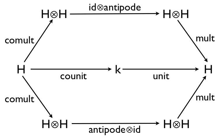
Recall that the definition requires that (mult . (id ⊗ antipode) . comult) == (unit . counit).

The left hand side is saying:
- first cut (deconcatenate) the deck of cards into two parts (in all possible ways)
- next apply the antipode to just one of the two parts
- finally shuffle the two parts together (in all possible ways)

The right hand side, remember, sends the empty permutation SSymF [] to itself, and every other permutation to zero.

So what this is saying is, you cut a (non-empty) deck of cards, wave a wand over one part, shuffle the two parts together again, and the cards all disappear!

Or is it? No, not quite. Remember that comult (resp. mult) is a sum of all possible deconcatenations (resp. shuffles). So what this is saying is that the antipode arranges things so that when you sum over all possible deconcatenations and shuffles, they cancel each other out. Cool!

(This sounds like it might have something to do with renormalization in physics, where we want to get a bunch of troublesome infinities to cancel each other out. There is apparently a connection between Hopf algebras and renormalization, but I don't know if this is it. Unfortunately my understanding of physics isn't up to figuring this all out.)


So we've now seen how to define Hopf algebra structures on two different sets of combinatorial objects: trees and permutations. We'll see that these two Hopf algebras are actually quite closely related, and that there is something like a family of combinatorial Hopf algebras with interesting connections to one another.

My main source for this article was Aguiar, Sottile, Structure of the Malvenuto-Reutenauer Hopf algebra of permutations.

Combinatorial Hopf Algebras I: The Hopf Algebra YSym of Binary Trees

Last time we looked at the definition of Hopf algebras, using the group algebra as a motivating example. This time I want to look at YSym, a Hopf algebra of binary trees. This is an example of a Combinatorial Hopf Algebra (CHA), meaning a Hopf algebra defined over some combinatorial object such as partitions, compositions, permutations, trees.

The binary trees we're concerned with are the familiar binary trees from computer science. In the math literature on this, however, they're called (rooted) planar binary trees. As far as I can tell, that's because in math, a tree means a simple graph with no cycles. So from that point of view, a CS binary tree is in addition rooted - it has a distinguished root node - and planar - so that you can distinguish between left and right child nodes.

Here's a Haskell type for (rooted, planar) binary trees:

data PBT a = T (PBT a) a (PBT a) | E deriving (Eq, Show, Functor)



instance Ord a => Ord (PBT a) where

    ...

As a convenience, the trees have labels at each node, and PBT is polymorphic in the type of the labels. The labels aren't really necessary: the Hopf algebra structure we're going to look at depends only on the shapes of the trees, not the labels. However, it will turn out to be useful to be able to label them, to see more clearly what is going on.

There's more than one way to set up a Hopf algebra structure on binary trees, so we'll use a newtype wrapper to identify which structure we're using.

newtype YSymF a = YSymF (PBT a) deriving (Eq, Ord, Functor)



instance Show a => Show (YSymF a) where

    show (YSymF t) = "F(" ++ show t ++ ")"



ysymF :: PBT a -> Vect Q (YSymF a)

ysymF t = return (YSymF t)

(The "F" in YSymF signifies that we're looking at the fundamental basis. We may have occasion to look at other bases later.)

So as usual, we're going to work in the free vector space on this basis, Vect Q (YSymF a), consisting of linear combinations of binary trees. Here's what a typical element might look like:

$ cabal update

$ cabal install HaskellForMaths

$ ghci

> :m Math.Algebras.Structures Math.Combinatorics.CombinatorialHopfAlgebra

> ysymF (E) + 2 * ysymF (T (T E () E) () E)

F(E)+2F(T (T E () E) () E)

Ok, so how do we multiply two binary trees together? Well actually, let's look at comultiplication first, because it's a little easier to explain. In CHAs (combinatorial Hopf algebras), the comultiplication is often a sum of the different ways of taking a combinatorial structure apart into two pieces. In the case of binary trees, we take them apart by splitting down the middle, starting at a leaf and continuing down to the root. Each node that we pass through goes to the side which has both its branches.

The diagram shows one possible split of the tree. Each leaf of the tree gives rise to a split. Hence the possible splits are:

> mapM_ print $ splits $ T (T E 1 E) 2 (T (T E 3 E) 4 (T E 5 E))

(E,T (T E 1 E) 2 (T (T E 3 E) 4 (T E 5 E)))

(T E 1 E,T E 2 (T (T E 3 E) 4 (T E 5 E)))

(T (T E 1 E) 2 E,T (T E 3 E) 4 (T E 5 E))

(T (T E 1 E) 2 (T E 3 E),T E 4 (T E 5 E))

(T (T E 1 E) 2 (T (T E 3 E) 4 E),T E 5 E)

(T (T E 1 E) 2 (T (T E 3 E) 4 (T E 5 E)),E)

The definition of splits is wonderfully simple:

splits E = [(E,E)]

splits (T l x r) = [(u, T v x r) | (u,v) <- splits l] ++ [(T l x u, v) | (u,v) <- splits r]

We use this to define a coalgebra structure on the vector space of binary trees as follows:

instance (Eq k, Num k, Ord a) => Coalgebra k (YSymF a) where

    counit = unwrap . linear counit' where counit' (YSymF E) = 1; counit' (YSymF (T _ _ _)) = 0

    comult = linear comult'

        where comult' (YSymF t) = sumv [return (YSymF u, YSymF v) | (u,v) <- splits t]

In other words, the counit is the indicator function for the empty tree, and the comult sends a tree t to the sum of u⊗v for all splits (u,v).

> comult $ ysymF $ T (T E 1 E) 2 (T E 3 E)

(F(E),F(T (T E 1 E) 2 (T E 3 E)))+(F(T E 1 E),F(T E 2 (T E 3 E)))+(F(T (T E 1 E) 2 E),F(T E 3 E))+(F(T (T E 1 E) 2 (T E 3 E)),F(E))

Let's just check that this satisfies the coalgebra conditions:

> quickCheck (prop_Coalgebra :: Vect Q (YSymF ()) -> Bool)

+++ OK, passed 100 tests.

[I should say that although the test code is included in the HaskellForMaths package, it is not part of the exposed modules, so if you want to try this you will have to fish around in the source.]

Multiplication is slightly more complicated. Suppose that we are trying to calculate the product of trees t and u. Suppose that u has k leaves. Then we look at all possible "multi-splits" of t into k parts, and then graft the parts onto the leaves of u (in order). This is probably easiest explained with a diagram:

The diagram shows just one possible multi-split, but the multiplication is defined as the sum over all possible multi-splits. Here's the code:

multisplits 1 t = [ [t] ]

multisplits 2 t = [ [u,v] | (u,v) <- splits t ]

multisplits n t = [ u:ws | (u,v) <- splits t, ws <- multisplits (n-1) v ]



graft [t] E = t

graft ts (T l x r) = let (ls,rs) = splitAt (leafcount l) ts

                     in T (graft ls l) x (graft rs r)



instance (Eq k, Num k, Ord a) => Algebra k (YSymF a) where

    unit x = x *> return (YSymF E)

    mult = linear mult'

        where mult' (YSymF t, YSymF u) = sumv [return (YSymF (graft ts u)) | ts <- multisplits (leafcount u) t]

For example:

> ysymF (T (T E 1 E) 2 E) * ysymF (T E 3 E)

F(T (T (T E 1 E) 2 E) 3 E)+F(T (T E 1 E) 3 (T E 2 E))+F(T E 3 (T (T E 1 E) 2 E))

It's fairly clear that the empty tree E is a left and right identity for this multiplication. It seems plausible that the multiplication is also associative - let's just check:

> quickCheck (prop_Algebra :: (Q, Vect Q (YSymF ()), Vect Q (YSymF ()), Vect Q (YSymF ())) -> Bool)

+++ OK, passed 100 tests.

So we've defined both algebra and coalgebra structures on the free vector space of binary trees. For a bialgebra, the algebra and coalgebra structures need to satisfy compatibility conditions: roughly, the multiplication and comultiplication need to commute, ie comult (mult x y) == mult (comult x) (comult y); plus similar conditions involving unit and counit.

Given the way they have been defined, it seems plausible that the structures are compatible (roughly, because it doesn't matter whether you split before or after grafting), but let's just check:

> quickCheck (prop_Bialgebra :: (Q, Vect Q (YSymF ()), Vect Q (YSymF ())) -> Bool)

+++ OK, passed 100 tests.

This entitles us to declare a Bialgebra instance:

instance (Eq k, Num k, Ord a) => Bialgebra k (YSymF a) where {}

(The Bialgebra class doesn't define any "methods". So this is just a way for us to declare in the code that we have a bialgebra. For example, we could write functions which require Bialgebra as a context.)


Finally, for a Hopf algebra, we need an antipode operation. Recall that an antipode must satisfy the following diagram:

In particular,

mult . (id ⊗ antipode) . comult = unit . counit

Let's assume that an antipode for YSym exists, and see what we can deduce about it. The right hand side of the above equation is the function that takes a linear combination of trees, and drops everything except the empty tree. Informally:
(unit . counit) E = E
(unit . counit) (T _ _ _) = 0

For example:

> (unit . counit) (ysymF E) :: Vect Q (YSymF ())

F(E)

> (unit . counit) (ysymF (T E () E)) :: Vect Q (YSymF ())

0

Since we also know that comult E = E⊗E, and mult E⊗E = E, it follows that antipode E = E.

Now what about the antipode of non-empty trees? We know that
comult t = E⊗t + ... + t⊗E
where the sum is over all splits of t.

Hence
((id ⊗ antipode) . comult) t = E⊗(antipode t) + ... + t⊗(antipode E)
and
(mult . (id ⊗ antipode) . comult) t = E * antipode t + ... + t * antipode E
where the right hand side of each multiplication symbol has antipode applied.

Now, E is the identity for multiplication of trees, so
(mult . (id ⊗ antipode) . comult) t = antipode t + ... + t * antipode E

Now, the Hopf algebra condition requires that (mult . (id ⊗ antipode) . comult) = (unit . counit). And we saw that for a non-empty tree, (unit . counit) t = 0. Hence:

antipode t + ... + t * antipode E = 0

Notice that all the terms after the first involve the antipodes of trees "smaller" than t (ie with fewer nodes). As a consequence, we can use this equation as the basis of a recursive definition of the antipode. We recurse through progressively smaller trees, and the recursion terminates because we know that antipode E = E. Here's the code:

instance (Eq k, Num k, Ord a) => HopfAlgebra k (YSymF a) where

    antipode = linear antipode'

        where antipode' (YSymF E) = return (YSymF E)

              antipode' x = (negatev . mult . (id `tf` antipode) . removeTerm (YSymF E,x) . comult . return) x

For example:

> antipode $ ysymF (T E () E)

-F(T E () E)

> antipode $ ysymF (T (T E () E) () E)

F(T E () (T E () E))



> quickCheck (prop_HopfAlgebra :: Vect Q (YSymF ()) -> Bool)

+++ OK, passed 100 tests.

It is also possible to give an explicit definition of the antipode (exercise: find it), but I thought it would be more illuminating to do it this way.

It's probably silly, but I just love being able to define algebraic structures on pictures (ie of trees).

Incidentally, I understand that there is a Hopf algebra structure similar to YSym underlying Feynman diagrams in physics.

I got the maths in the above mainly from Aguiar, Sottile, Structure of the Loday-Ronco Hopf algebra of trees. Thanks to them and many other researchers for coming up with all this cool maths, and for making it freely available online.

What is a Hopf algebra?

A while ago I looked at the concepts of an algebra and a coalgebra, and showed how to represent them in Haskell. I was intending to carry on to look at bialgebras and Hopf algebras, but I realised that I wasn't sufficiently clear in my own mind about the motivation for studying them. So, I confess that I have been keeping this blog just about afloat with filler material, while behind the scenes I've been writing loads of code - some fruitful, some not - to figure out how to motivate the concept of Hopf algebra.

Some concepts in mathematics have an obvious motivation at the outset: groups arise from thinking about (eg geometric) symmetry, (normed) vector spaces are a representation of physical space. (Both concepts turn out to have a usefulness that goes far beyond the initial intuitive motivation.) With Hopf algebras this doesn't really appear to be the case.

Hopf algebras appear to have been invented for narrow technical reasons to solve a specific problem, and then over time, it has turned out both that they are far more widespread and far more useful than was initially realised. So for me, there are two motivations for looking at Hopf algebras:
- There are some really interesting structures that are Hopf algebras. I'm particularly interested in combinatorial Hopf algebras, which I hope to cover in this blog in due course. But there are also examples in physics, associated with Lie algebras, for example.
- They have some interesting applications. I'm interested in the applications to knot theory (which unfortunately are a little technical, so I'll have to summon up some courage if I want to go over them in this blog). But again, there seem to be applications to physics, such as renormalization in quantum field theory (which I don't claim to understand, btw).


As a gentle introduction to Hopf algebras, I want to look at the group Hopf algebra, which has some claim to be the fundamental example, and provides a really good anchor for the concept.

So last time we looked at the group algebra - the free k-vector space of k-linear combinations of elements of a group G. We saw that many elements in the group algebra have multiplicative inverses, and we wrote code to calculate them. However, if you look again at that code, you'll see that it doesn't actually make use of group inverses anywhere. The code really only relies on the fact that finite groups are finite monoids. We could say that actually, the code we wrote is for finding inverses in finite monoid algebras. (But of course it just so happens that all finite monoids are groups.)

[Edit: Oops - that last claim in brackets is not true. Thanks to reddit readers for pointing it out.]

So the group algebra is an algebra, indeed a monoid algebra, but with the special property that the basis elements (the group elements) all have multiplicative inverses.

Now, mathematicians always prefer, if possible, to come up with definitions that are basis-independent. (In HaskellForMaths, we've been working with free vector spaces, which encourages us to think of vector spaces in terms of a particular basis. But many interesting properties of vector spaces are true regardless of the choice of basis, so it is better to find a way to express them that doesn't involve the basis.)

Can we find a basis-independent way to characterise this special property of the group algebra?

Well, our first step has to be to find a way to talk about the group inverse without having to mention group elements. We do that by encapsulating the group inverse in a linear map, which we call the antipode:

antipode x = nf (fmap inverse x)

So in other words the antipode operation just inverts each group element in a group algebra element (a k-linear combination of group elements). (The nf call just puts the vector in normal form.) For example:

> antipode $ p [[1,2,3]] + 2 * p [[2,3,4]]
[[1,3,2]]+2[[2,4,3]]

The key point about the antipode is that we now have a linear map on the group algebra, rather just an operation on the group alone. Although we defined the antipode in terms of a particular basis, linear maps fundamentally don't care about the basis. If you choose some other basis for the group algebra, I can tell you how the antipode transforms your basis elements.


Ok, so what we would like to do is find a way to express the group inverse property (ie the property that every group element has an inverse) as a property of the group algebra, in terms of the antipode.

Well, no point beating about the bush. Define:

trace (V ts) = sum [x | (g,x) <- ts]
diag = fmap (\g -> (g,g))

(So in maths notation, diag is the linear map which sends g to g⊗g.)

Note that these are both linear maps. In particular, once again, although we have defined them in terms of our natural basis (the group elements), as linear maps they don't really care what basis we choose.


Then it follows from the group inverse property that the following diagram commutes:

Why will it commute? Well, think about what happens to a group element, going from left to right:
- Going along the top, we have g -> g⊗g -> g⊗g^-1 -> g*g^-1 = 1
- Going along the middle, we have g -> 1 -> 1
- Going along the bottom, we have g -> g⊗g -> g^-1⊗g -> g^-1*g = 1
All of the maps are linear, so they extend from group elements to arbitrary k-linear combinations of group elements.

(Shortly, I'll demonstrate that it commutes as claimed, using a quickcheck property.)


We're nearly there. We've found a way to express the special property of the group algebra, in a basis-independent way. We can say that what is special about the group algebra is that there is a linear antipode map, such that the above diagram commutes.

[In fact I think it may be true that if you have a monoid algebra such that the above diagram commutes, then it follows that the monoid is a group. This would definitely be true if we constrained antipode to be of the form (fmap f), for f a function on the monoid, but I'm not absolutely sure that it's true if antipode is allowed to be an arbitrary linear function.]

Now, the concept of a Hopf algebra is just a slight generalization of this.

Observe that trace and diag actually define a coalgebra structure:
- diag is clearly coassociative
- the left and right counit properties are also easy to check

So we can define:

instance (Eq k, Num k) => Coalgebra k (Permutation Int) where

    counit = unwrap . linear counit' where counit' g = 1  -- trace

    comult = fmap (\g -> (g,g))                           -- diagonal

(In fact, trace and diag define a coalgebra structure on the free vector space over any set. Of course, some free vector spaces also have other more interesting coalgebra structures.)

Let's just quickcheck:

> quickCheck (prop_Coalgebra :: GroupAlgebra Q -> Bool)
+++ OK, passed 100 tests.


So for the definition of a Hopf algebra, we allow the antipode to be defined relative to other coalgebra structures besides the trace-diag structure (with some restrictions to be discussed later). So a Hopf algebra is a vector space having both an algebra and a coalgebra structure, such that there exists an antipode map that makes the following diagram commute:

Thus we can think of Hopf algebras as a generalisation of the group algebra. As we'll see (in future posts), there are Hopf algebras with rather more intricate coalgebra structures and antipodes than the group algebra.

Here's a Haskell class for Hopf algebras:

class Bialgebra k b => HopfAlgebra k b where

    antipode :: Vect k b -> Vect k b

(A bialgebra is basically an algebra plus coalgebra - but with one more condition that I'll explain in a minute.)

We've already seen the antipode for the group algebra, but here it is again in its proper home, as part of a Hopf algebra instance:

instance (Eq k, Num k) => HopfAlgebra k (Permutation Int) where

    antipode = nf . fmap inverse

And here's a quickCheck property:

prop_HopfAlgebra x =

    (unit . counit) x == (mult . (antipode `tf` id) . comult) x &&

    (unit . counit) x == (mult . (id `tf` antipode) . comult) x



> quickCheck (prop_HopfAlgebra :: GroupAlgebra Q -> Bool)

+++ OK, passed 100 tests.

So there you have it. That's what a Hopf algebra is.

Except that I've cheated slightly. What I've defined so far is actually only a weak Hopf algebra. There is one other condition that is needed, called the Hopf compatibility condition. This requires that the algebra and coalgebra structures are "compatible" in the following sense:
- counit and comult are algebra morphisms
- unit and mult are coalgebra morphisms

I don't want to dwell too much on this. It seems a pretty reasonable requirement, although other compatibility conditions are possible (eg Frobenius algebras). An algebra plus coalgebra satisfying these conditions (even if it doesn't have an antipode) is called a bialgebra. And it turns out that the group algebra is one.

> quickCheck (prop_Bialgebra :: (Q, GroupAlgebra Q, GroupAlgebra Q) -> Bool)
+++ OK, passed 100 tests.